I will introduce you to Colab from Google Drive: the basics, a few useful links, useful tips and procedures.
Summary
Brief overview and advantages
Useful start
Access to resources
Shell and R
Scratch cells
Google drive and packages
Final tips
Code example
Useful references
Summary...
Colab
Advantages
From google drive: all advantages of drive document
Free RAM, CPU, GPU (limited resources and time)
No installation needed
Online interface, cloud-based runtime
A lot of tutorials and documentation
Settings
Python language as default
easy acces to sh and R oneliners
Availability of R kernel
Markdown format
Hierarchies
Collapse cells to run multiple chunks at once
Code, scratch, text cells
It is temporal
Objects and files (binary files for installed libraries) will be lost
Take advantage of google drive access to save objects and libraries
Brief overview and advantages
Google Colaboratory is a tool used to edit, save, execute, and share python code via Google Drive. The colab notebook has similar properties to any other google drive document, you can create/share/download/upload it through that website (Fig. 1). One of the most remarkable advantages of Colab is that it provides you the opportunity to run code with the Google computational resources. Even the free version has competitive amounts of RAM/processors including access to GPUs. I have used this version to perform some basic metagenomic, scRNA-seq, statistical and machine learning analysis, although it has a lower amount of RAM and CPUs than most PBS, it was a better option than my regular laptop, maybe it is for you too. The other attractive feature of Colab is its user-friendly feature. It is perfect for beginners, you only need an internet connection, and the python environment would be available for you; forget about wasting your computational resources and time in the installation of python/conda/text editors. Finally, you can access it even from your phone, however, its design is easier to use in computers.
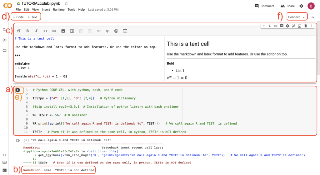
The Colab documents have a Jupyter notebook format (Fig. 2); this means that you can combine code, text, rich media, etc. in an interactive and executable document. In these documents, the content is divided by cells, which allows you to have a more structured, organised, and easy to read code. There are two classes of cells, the more important type is the code cell (Fig. 2a). As its name suggests, it is used to write and execute code as if you were writing code in any terminal. For colab, the default language in these cells is python. However, you can combine bash and R oneliners in the same cell with python code; just consider that R and bash variables will not be available in python (Fig. 2b). Then, there are the text cells (Fig 2c), such cells have a markdown syntax, these are usually used to provide a narrative to your code and allows you to include images, latex formulas, structured data, etc. Using the buttons in Fig. 2d is the easiest way to add any of these cells. Finally, the Jupyter format allows you to use the same document either in Jupyter or colab.
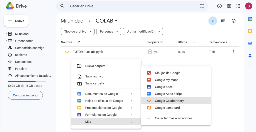
Figure 1. Colab is integrated in google drive. You can save/access/create/edit/upload/download/share colab notebooks with .ipynb format with google drive as you can do it with any other document. TUTORIALcolab is an example of a colab notebook.
The Colab notebook format
The Colab documents have a Jupyter notebook format (Fig. 2); this means that you can combine code, text, rich media, etc. in an interactive and executable document. In these documents, the content is divided by cells, which allows you to have a more structured, organised, and easy to read code. There are two classes of cells, the more important type is the code cell (Fig. 2a). As its name suggests, it is used to write and execute code as if you were writing code in any terminal. For colab, the default language in these cells is python. However, you can combine bash and R oneliners in the same cell with python code; just consider that R and bash variables will not be available in python (Fig. 2b). Then, there are the text cells (Fig 2c), such cells have a markdown syntax, these are usually used to provide a narrative to your code and allows you to include images, latex formulas, structured data, etc. Using the buttons in Fig. 2d is the easiest way to add any of these cells. Finally, the Jupyter format allows you to use the same document either in Jupyter or colab.
Figure 2. Overview of a colab notebook. The notebook is composed of (a) code and text (c) cells. The default language is python, but you can combine different languages. In (b), we define the TESTr variable using a one liner of R, such variable is saved in the R kernel, but TESTr is not found in the python kernel (b). For text cells (c), the editor is on the left side of, while a preview is shown on the left. Any of these cells can be added by clicking (d). On a recently opened notebook, we can access the computational resources by clicking on the (e) run (f) or connect button.
Useful start
If you haven’t used colab and you are interested, the colab welcome document is a very good start. It has an excellent overview of the product and links to useful tutorials. In this post I am going to recover a pair of components of the welcome document and additional features that can be useful for you. On the other hand, the seedbank repository has multiple examples of python codes with the availability of use colab to visualise them, this may give you an idea of how to use colab.
A brief overview of the access to resources in colab
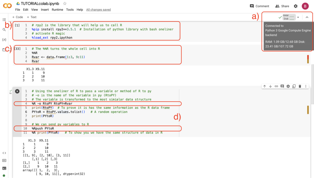
Before I continue, I want to emphasise one more time that Colab has a cloud-based runtime. You can load your runtime by clicking the connect button at the top right of the notebook (Fig 2f), or by running a cell (Fig. 2e). All cells have the same runtime, therefore, any variable saved in the cell X of your document can be used in the cell Y. On the other hand, you can click the run button on all cells at once, but the first cell must finish before the second starts to process its code. You also can link colab to your local machine, but that is optional. The Google computational resources in colab are limited and depend on availability, time, pattern of use of the user, etc. At the top right of the notebook, you can look at a wide overview of your available resources (Fig. 3a). On the other hand, colab is expected to be interactive, therefore you can not let your 3 days script running without supervision. At most, you can use the same runtime for even 12 hours in the free version (up to 24 hours in the paid reservation). At least in the free version, depending on the available resources, colab can finish your runtime before the 12 hours, I had runs for which colab closed my runs after 5 hours I did not interact with the notebook. Finally, the paid version gives you more resources, but even in this version we have restrictions.
Shell and R languages in colab
Colab was designed to write python code and it easily adapts some sh commands. To do it, you only need to add a percentage symbol (%) prior to any shell command; the expression symbol (!)can also be used to run shell commands, but it uses a subshell cell and the results are not permanent in the python kernel (Fig. 3b, 2a). This syntax will allow you to install python packages. Some time ago, colab implemented a R kernel, if you access the notebook through a link or by configuring your kernel (more info), you will be able to run R code in more than one line. However, I have not found the right way to mount my google drive folder in the runtime to access my data. Thankfully, we have another option though it is less elegant, the R magic library. You can use the rpy2.ipython library (Fig. 3b). At least on March 23 colab required the rpy2==3.5.1 package version to use R magic; you can try it if you have problems using it. As a brief overview, once you install the library, just add %%R to use the whole cell with R code (Fig 3c). Adding just one percentage symbol (%R) is for one liners (Fig. 2a). I know combining languages is not the most suitable decision most of the time, but, if you already took that path, you may want to use some additional commands. You can exchange some equivalent R and python variables with the codes in Fig. 3d.
Figure 3. Computational/language resources. a) Overview of your computational resources, it appears once you are connected. b) Use this library to access magic R. c) Using %%R turns the whole cell to R. d) You can exchange variables between kernels.
Temporal/scratch code cells
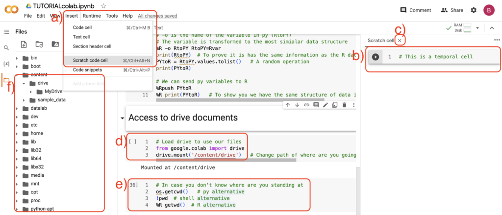
One simple, but cool thing about colab is the temporal/scratch code cell. This type of cell can be used to test code lines, or to run code that you do not want to include in your final script. To get access to it you can click the button Insert -> Scratch code cell (Fig 4a). After this, a new tab will open at the colab document (4b). Such a tab has the same runtime as the others, but it is a little easier to break, only click x (Fig 4c). I like to use this cell when I use R magic since these codes are difficult to stop in the regular cells. If I make a mistake or the output is longer than expected, I can either wait until the run finishes or disconnect and clean all the execution environment which means I would have to run everything again. On the other hand, temporal cells will finish R runs yes or yes if I close the temporal tab.
Figure 4. Temporal cells and the access to drive documents. Inset -> Scratch code cell (a)l opens a temporal cell (b) that can be easily closed by clicking (c). To have access to your google drive documents, follow the steps in (d), you would have to confirm the access in an emergent tab. e) code will help you to know where you are standing. f) is the graphical display of your directories, in this example, My drive has my drive’s documents.
Mount your google drive documents and saving your installed packages: A countermeasure to keep your progress
Now, let’s talk about one of the most annoying aspects of colab. As happens with Jupyter, if you close the colab notebook or your runtime is disconnected, the image of the results in each cell will be saved until you re-run the code. However, in colab you will not only lose any object, and data in your environment, you will also lose your installed packages. To counter that issue, you can mount your google drive directory in google colab and save your main results as tables, or binary objects (pickle.load library for py, saveRDS() command for R). I have not used Google Drive in other python interfaces; however, I can tell you that mounting your drive documents in colab is very easy. You only need to run the code in Fig. 4d, follow the steps to select and give access to your account, then you would have access to your Google Drive documents from colab. The graphical overview of this is located at the left side of the notebook: folder icon -> my drive -> MyDrive (4d). If you have doubts about your current location, you can use (!pwd) as in shell, or any other variant in other languages (Fig. 4e).
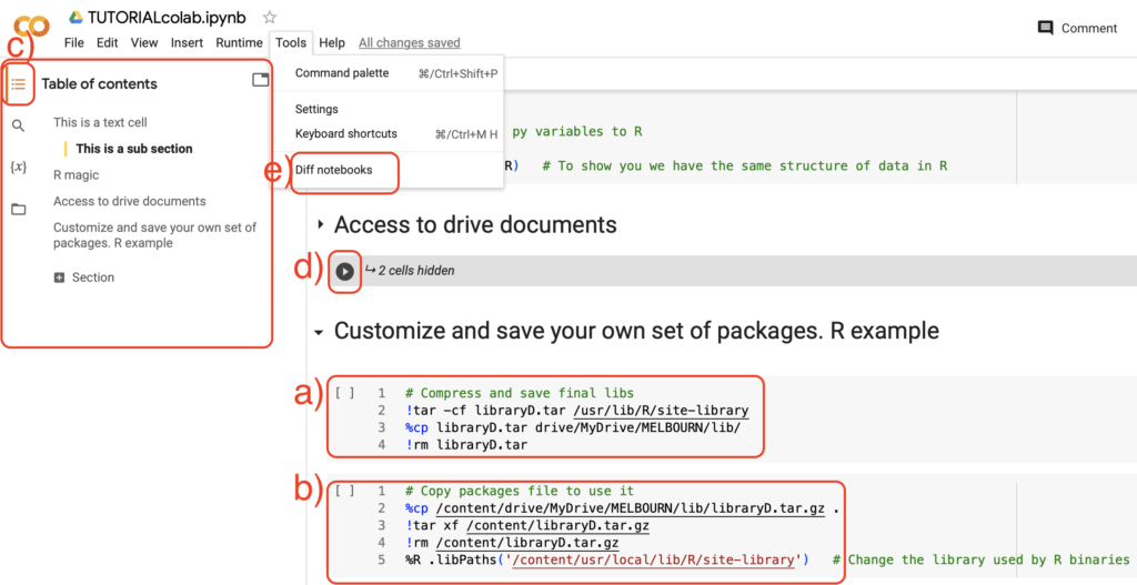
Figure 5. Packages configuration saving and additional features. Use the steps in a) to avoid re-installing the same packages over and over again. Use the code in b) to retrieve such packages. Take advantage of the hierarchy of the markdown. You can group cell and text cells, the overview is in (c). This will allow you to have order and to execute a set of cells that are grouped together all at once (d).
On the other hand, Sometimes the installation of packages can take as much time as running your code. My best advice if your package installation process takes too long is to save the binaries of your packages. Just be careful because depending on the case, this may consume more memory. To do it, first locate where your binaries are saved, then compress these files and copy them to your google drive account (Fig. 5a). If you want to use them again, make the inverse process (Fig. 5b). Regarding packages, I have final advice, avoid as much as possible to rewrite already installed packages. In my experience, I find it best to explore the multiple R library folders to see which one was more complete and install my new packages at that location.
Final basic advises when using colab
Use the markdown syntax to have your code organised and hierarchized by headers. If the length of your document increases, this practice will allow you to locate and select in the index your sections of interest (Fig. 5c). Besides, you can choose at what level you display (expand) your cells and that allows you to choose the scale at which you read your document. Plus, if you group cells by headers, you can contract those cells in a single section and run the whole section at once (Fig. 6d).
Make sure you save the changes. Most of the time, colab will save your changes automatically. However, sometimes you will have to click ctrl + S to manually save it and colab will show you a popup to inform you that your changes have not been saved yet. Opening the same notebook more than once is the easiest way to get that pop up, avoid it as much as possible. In Tools -> Diff notebooks you can visualise the last versions of your notebook and compare them with the current version.
Be aware of your location. If you are going to mount google drive, be sure you are saving/uploading your archives to/from the right location.
If your RAM is consumed in the first try, give it another try. I do not have the right explanation for this, but I have been in the situation where I run a set of heavy code lines and the RAM is consumed entirely, then I reset the runtime (clear and reset environment), I run the same code lines and now I have enough RAM. This may be a consequence of the constantly changing availability of resources of colab. Therefore, I encourage you to keep an open mind.
Follow the river with libraries incompatibilities. As I stated before, I would recommend prioritizing keeping the original colab packages. On the other hand, you can always visit stack overflow to know your best option.
Use gc() and keep your environment clean. Since we have limited resources in the colab, try to use functions, delete unused variables and release the inaccessible data with gc.
Keep ready for changes. Colab is in constant development. You must be prepared for upgrades to packages, changes in resources availability, etc. You must keep updated to be able to use it for a long time.
Use clean and disconnect runtime. You may see different options to clean your environment, but just the clean and disconnect option will release your computational resources.
We use cookies on our website to give you the most relevant experience by remembering your preferences and repeat visits. By clicking “Accept All”, you consent to the use of ALL the cookies. However, you may visit "Cookie Settings" to provide a controlled consent.
This website uses cookies to improve your experience while you navigate through the website. Out of these, the cookies that are categorized as necessary are stored on your browser as they are essential for the working of basic functionalities of the website. We also use third-party cookies that help us analyze and understand how you use this website. These cookies will be stored in your browser only with your consent. You also have the option to opt-out of these cookies. But opting out of some of these cookies may affect your browsing experience.
Necessary cookies are absolutely essential for the website to function properly. These cookies ensure basic functionalities and security features of the website, anonymously.
Cookie
Duration
Description
cookielawinfo-checkbox-analytics
11 months
This cookie is set by GDPR Cookie Consent plugin. The cookie is used to store the user consent for the cookies in the category "Analytics".
cookielawinfo-checkbox-functional
11 months
The cookie is set by GDPR cookie consent to record the user consent for the cookies in the category "Functional".
cookielawinfo-checkbox-necessary
11 months
This cookie is set by GDPR Cookie Consent plugin. The cookies is used to store the user consent for the cookies in the category "Necessary".
cookielawinfo-checkbox-others
11 months
This cookie is set by GDPR Cookie Consent plugin. The cookie is used to store the user consent for the cookies in the category "Other.
cookielawinfo-checkbox-performance
11 months
This cookie is set by GDPR Cookie Consent plugin. The cookie is used to store the user consent for the cookies in the category "Performance".
viewed_cookie_policy
11 months
The cookie is set by the GDPR Cookie Consent plugin and is used to store whether or not user has consented to the use of cookies. It does not store any personal data.
Functional cookies help to perform certain functionalities like sharing the content of the website on social media platforms, collect feedbacks, and other third-party features.
Performance cookies are used to understand and analyze the key performance indexes of the website which helps in delivering a better user experience for the visitors.
Analytical cookies are used to understand how visitors interact with the website. These cookies help provide information on metrics the number of visitors, bounce rate, traffic source, etc.
Advertisement cookies are used to provide visitors with relevant ads and marketing campaigns. These cookies track visitors across websites and collect information to provide customized ads.